
This blog post is part of the Supercharging your large ClickHouse data loads series:
Going on a race track
In this second part of our three-part blog series about supercharging large data loads, we will put the theory from the first post into practice by demonstrating how you can run a large multi-billion row insert 3 times faster than with default settings using the same hardware. We outline a formula that you can use to determine the best block size / parallelism ratio for your ingestion use case. And lastly, we will break the speed limit by utilizing ClickHouse Cloud’s new SharedMergeTree table engine combined with easy horizontal cluster scaling.
Note that we only demonstrate a tuning scenario here, where data is pulled by the ClickHouse servers themselves. You can read about a setting where clients push the data to ClickHouse here.
The challenge
Using ClickHouse for large data loads is like driving a high-performance Formula One car 🏎 . A copious amount of raw horsepower is available, and you can reach top speed for your large data load. But, to achieve maximum ingestion performance, you must choose (1) a high enough gear (insert block size) and (2) an appropriate acceleration level (insert parallelism) based on (3) the concrete amount of available horsepower (CPU cores and RAM).
Ideally, we would like to drive our race car in the highest gear with full acceleration:
- Highest gear: The larger we configure the insert block size, the fewer parts ClickHouse has to create, and the fewer disk file i/o and background merges are required.
- Full acceleration: The higher we configure the number of parallel insert threads, the faster the data will be processed.
However, there is a conflicting tradeoff between these two performance factors (plus a tradeoff with background part merges). The amount of available main memory of ClickHouse servers is limited. Larger blocks use more main memory, which limits the number of parallel insert threads we can utilize. Conversely, a higher number of parallel insert threads requires more main memory, as the number of insert threads determines the number of insert blocks created in memory concurrently. This limits the possible size of insert blocks. Additionally, there can be resource contention between insert threads and background merge threads. A high number of configured insert threads (1) creates more parts that need to be merged and (2) takes away CPU cores and memory space from background merge threads.
Our challenge is to find a sweet spot with a large enough block size and a large enough number of parallel insert threads to reach the best possible insert speed.
The experiment
In the following sections, we put these block size / parallelism settings to the test and evaluate their effect on ingest speed.
Test data
The data we experiment with is from the PyPi dataset (hosted in a GCS bucket). It consists of 65.33 billion rows and has a raw, uncompressed size of ~14 TiB. The compressed data size on disk (when stored in a ClickHouse table) is ~1.2 TiB.
Test table and insert query
For these tests, we will ingest this data as fast as possible into a table in a ClickHouse Cloud service that consists of 3 ClickHouse servers with 59 CPU cores and 236 GiB of RAM per server. We’ll use an INSERT INTO SELECT query in combination with the s3Cluster integration table function (which is compatible with gcs).
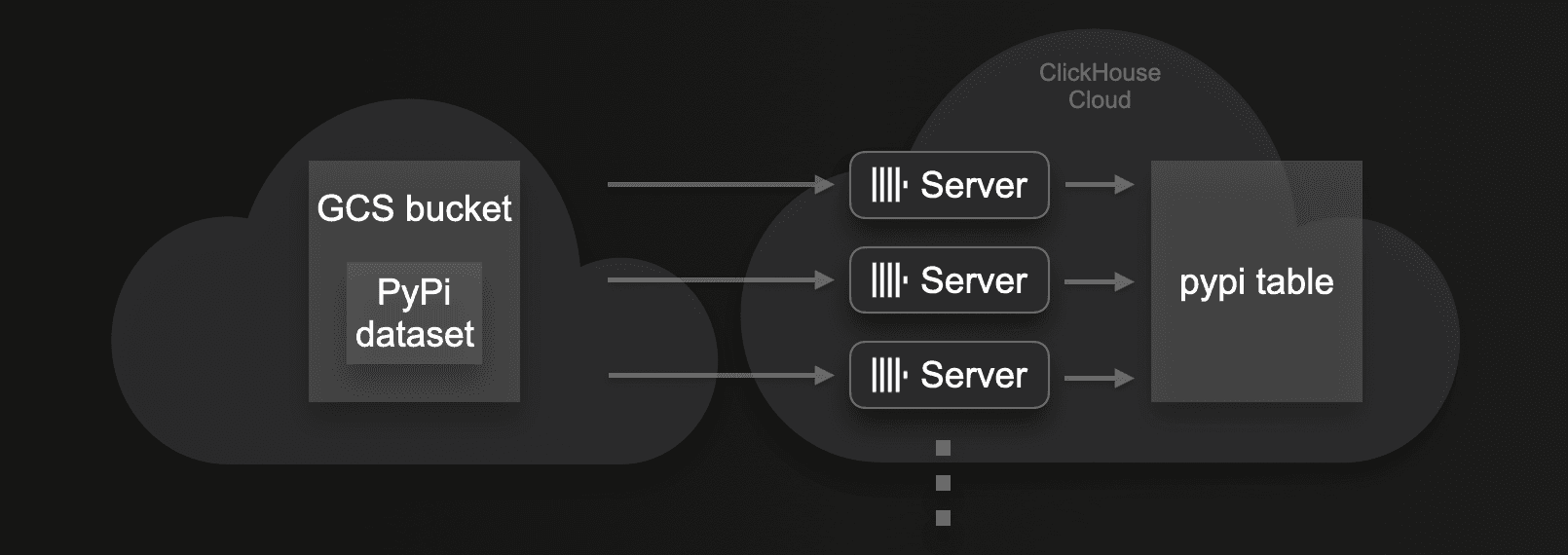
We’ll start by ingesting our large dataset with the default settings for insert block size and insert threads, and will then repeat this load with different numbers to assess the impact on load time.
Queries for introspecting performance metrics
We are using the following SQL queries over system tables for introspecting insert performance metrics visualized in our test results:
- Number of active parts at ingest finish
- Time to reach less than 3k active parts
- Number of initial parts written to storage
- Number of initial parts written to storage per cluster node
Shifting gears

To illustrate how insert block sizes impact the number of parts that get created (and need to be merged), we visualize below various insert block sizes (in terms of rows) versus the (uncompressed) average in-memory size of a single data block and its corresponding (compressed) average on-disk size of a single data part. This is overlayed with the average overall number of parts written to storage. Note that we give average values because, as mentioned in the first post, the created blocks and parts rarely precisely contain the configured number of rows or bytes, as ClickHouse is streaming and processing data row-block-wise. Therefore these settings specify minimum thresholds.
Also, note that we took these numbers from the results of different ingest test runs in the next section.
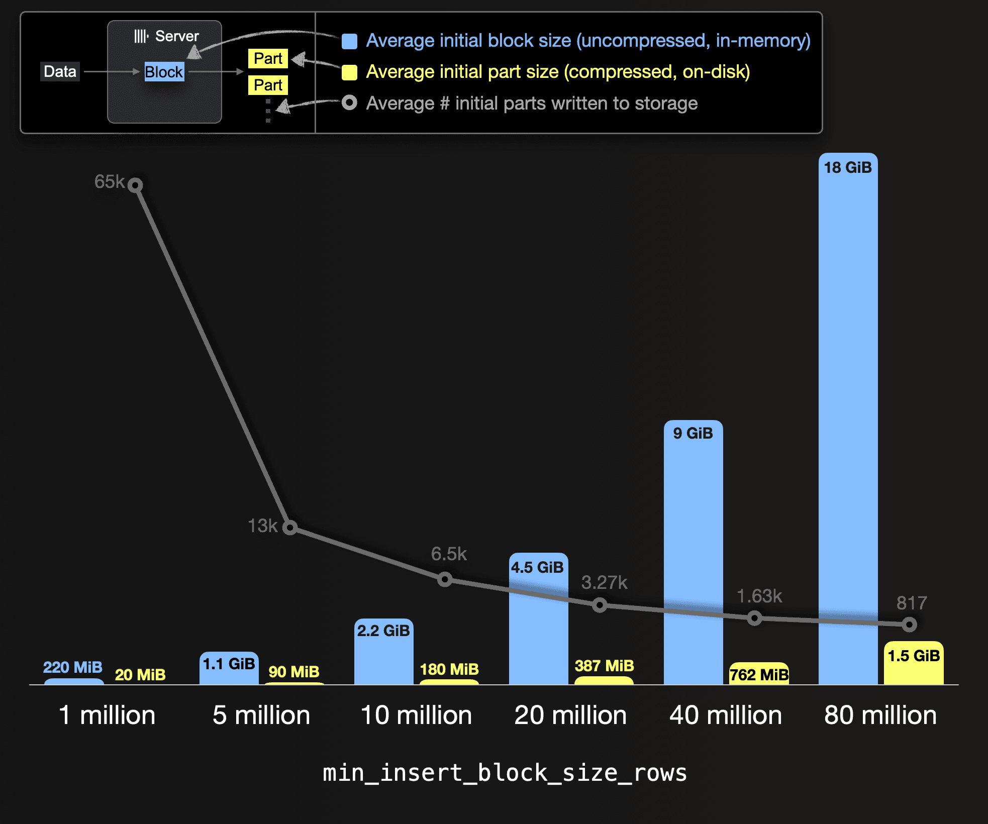 You can see that the larger we configure the insert block size, the fewer parts need to be created (and merged) for storing the test data, ~1.2 TiB of compressed table data. For example, with an insert block size of 1 million rows, 65 thousand initial parts (with an average compressed size of 20 MiB) will be created on disk. Whereas with an insert block size of 80 million rows, only 817 initial parts get created (with an average compressed size of 1.5 GiB).
Standard speed
The following chart visualizes the result of ingest runs with the default insert block size of ~1 million rows but different numbers of insert threads. We show the peak memory used and the resulting time for the number of parts to reach 3000 (the recommended number for efficient querying):
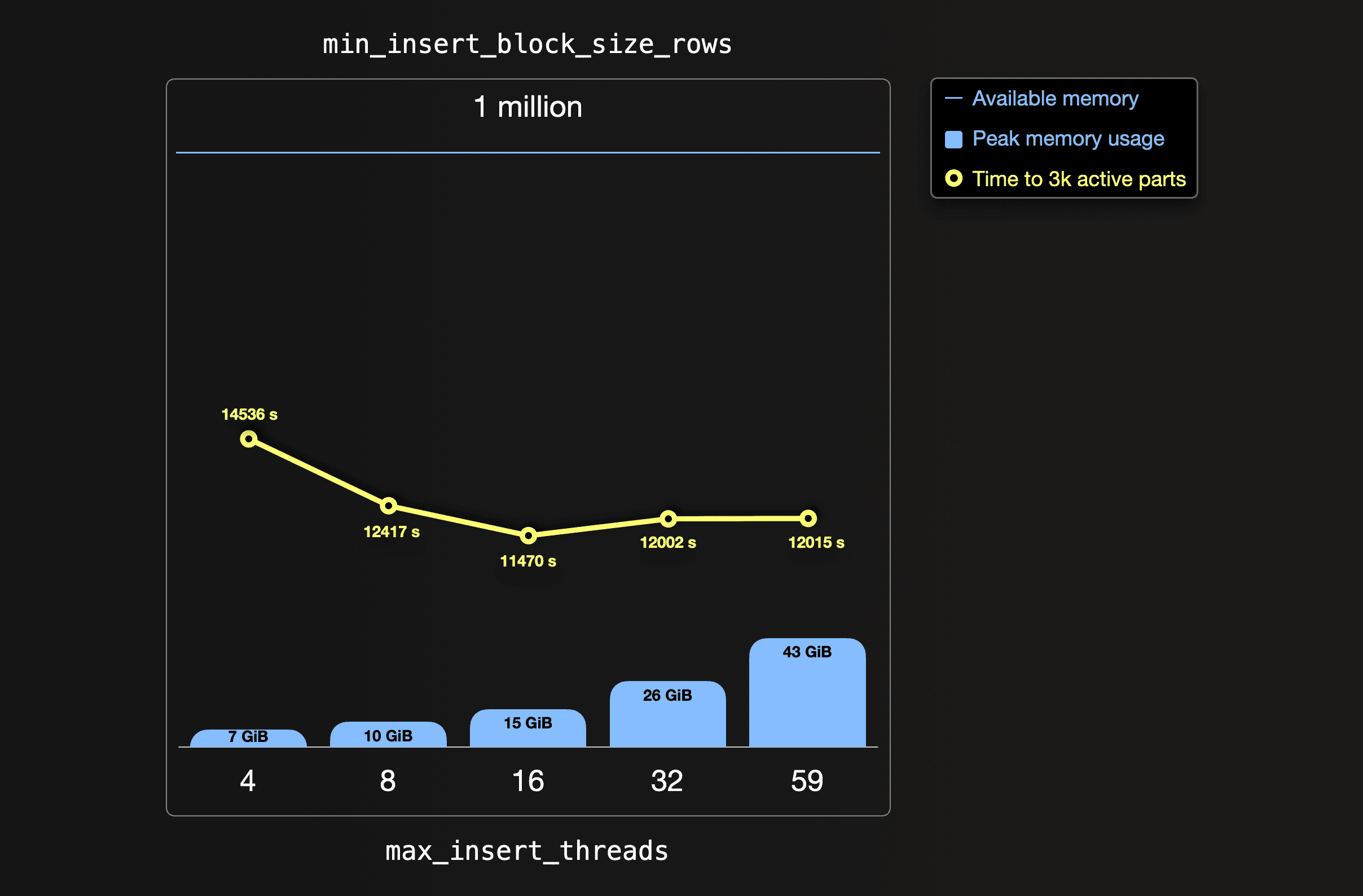 With the ClickHouse Cloud default setting of 4 ingest threads (default is no parallel ingest threads in OSS), the peak amount of consumed main memory is 7 GiB per server. It takes over 4 hours from the start of the ingest until the 65 thousand initially created parts are merged to a healthy number of less than 3 thousand parts. With its default settings, ClickHouse tries to offer a good balance of resource usage for supporting concurrent tasks from concurrent users. One size doesn’t fit all, though. Our goal here is to tune a dedicated service only used by us for one purpose: Achieving top speed for inserting our dataset.
If we match the amount of utilized parallel insert threads with the number of 59 available CPU cores, the time to 3k active parts is increased compared to lower thread settings.
The lowest time is achieved with 16 insert threads, leaving plenty of the 59 CPU cores available for background part merge threads that run concurrently with the data insertion.
Note that the blue horizontal bar on top in the chart above denotes the available memory per server (236 GiB RAM). We can see that there is much room for increasing insert block size and memory usage (blue vertical bars in the chart above), respectively.
Currently, we are pushing the accelerator pedal with full force (up to 59 insert threads) in a very low gear (only 1 million rows per initial part), resulting in a low overall ingestion speed. We will now find a better gear and acceleration combination in the next section.
Top speed

We tried to identify the perfect combination of insert block size and number of insert threads by running ingestions with different systematic combinations for these insert speed factors. The following chart visualizes the results of these ingest test runs, where we doubled the insert block size a few times (from 1 million to 5 million to 10 million to 20 million to 40 million, until 80 million):
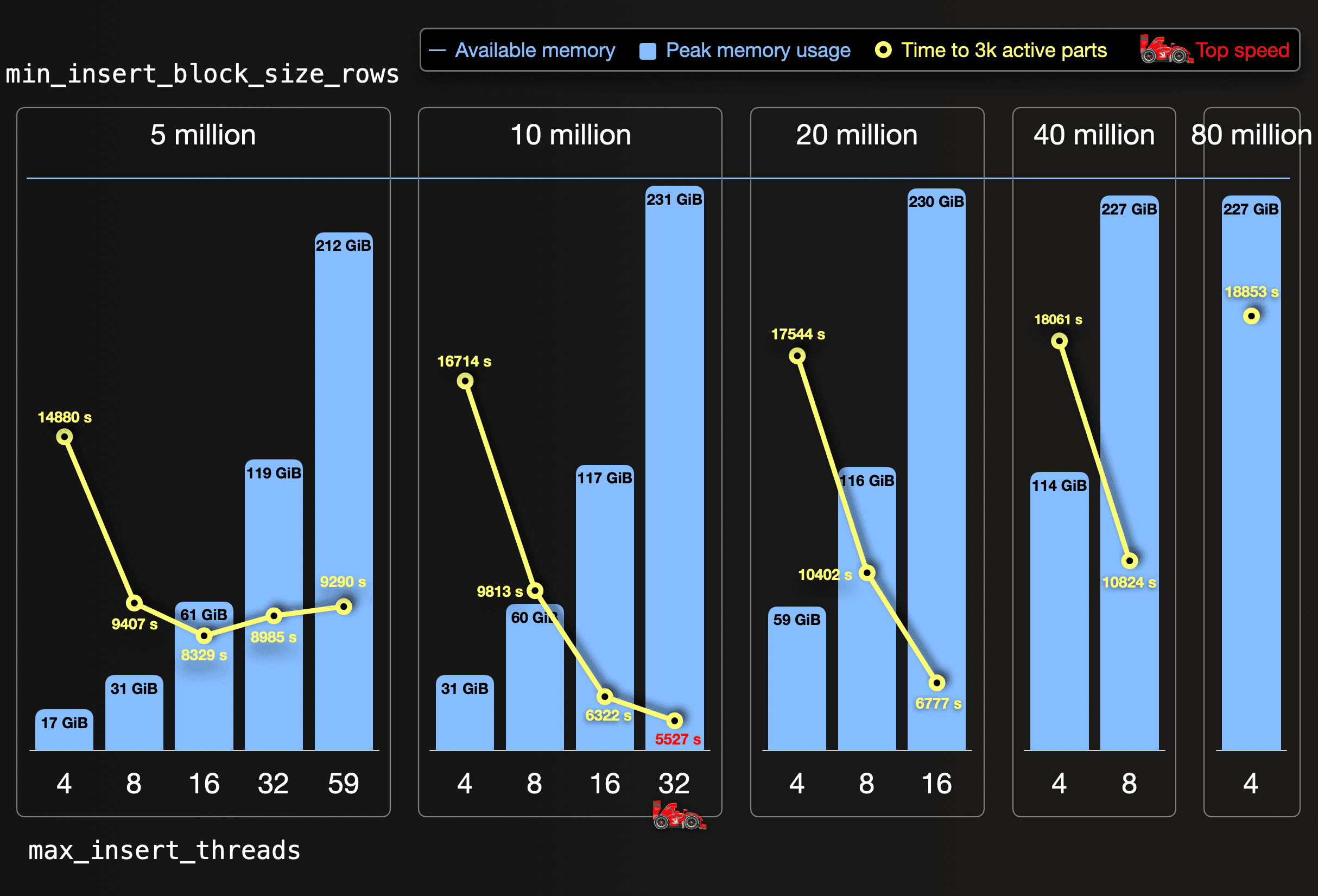
For each block size, we doubled the number of insert threads (starting at 4) until the peak memory usage (blue vertical bars) almost reached the available memory per server (blue horizontal bar). The yellow circles indicate the time from the start of the ingest until all initially created parts are merged to a healthy number of less than 3000 parts.
We reached top speed when the 65.33 billion rows of our dataset were ingested by 32 parallel insert threads with an insert block size of 10 million rows. This is the sweet spot for our server size of 59 CPU cores and 236 GiB RAM. This causes a moderate amount of 6.5 thousand initial parts, that can be quickly merged to less than 3000 parts in the background by the free 27 CPU cores (32 cores are used for reading and ingesting the data in parallel). With 16 insert threads and less, the insert parallelism is too low. With 59 insert threads, a 10 million rows block size doesn’t fit into the RAM.
A 5 million row block size works with 59 insert threads. Still, it creates 13 thousand initial parts without leaving any dedicated CPU cores for an efficient background merging, resulting in resource contention and a long time to reach 3 thousand active parts. With 32 and 16 insert threads, the data is processed slower but merged faster as more dedicated CPU cores are available for background merges. 4 and 8 insert threads don’t create enough insert parallelism with a 5 million row block size.
Insert block sizes of 20 million rows and more cause low numbers of initial parts, but the high memory overhead restricts insertion to a low number of insert threads creating insufficient insert parallelism.
With our identified sweet spot settings, we sped up the ingest by a factor of almost 3. We used exactly the same underlying hardware, but we utilized it more effectively for our data ingestion, without creating too many initial parts by pressing the accelerator pedal in half force (32 insert threads) with the highest possible gear (10 million rows block size).
Formula One
We are aware that identifying perfect settings for large multi-billion row inserts via several test runs is impractical. Therefore we give you this handy formula for calculating approximately the settings for top speed of your large data loads:
• max_insert_threads: choose ~ half of the available CPU cores for insert threads (to leave enough dedicated cores for background merges)
• peak_memory_usage_in_bytes: choose an intended peak memory usage; either all available RAM (if it is an isolated ingest) or half or less (to leave room for other concurrent tasks)
Then:min_insert_block_size_bytes = peak_memory_usage_in_bytes / (~3 * max_insert_threads)
With this formula, you can set min_insert_block_size_rows to 0 (to disable the row based threshold) while setting max_insert_threads to the chosen value and min_insert_block_size_bytes to the calculated result from the above formula.
Breaking the speed limit with ClickHouse Cloud

The next measure to make the ingestion even faster is to put more horsepower into our engine and increase the number of available CPU cores, respectively, by adding additional servers.
Combined with its SharedMergeTree table engine, ClickHouse Cloud allows you to freely (and quickly!) either change the size (CPU and RAM) of existing servers or add additional servers. We did the latter with our service and ingested our dataset with different numbers of ClickHouse servers (each with 59 CPU cores and 236 GB RAM). This chart shows the results:
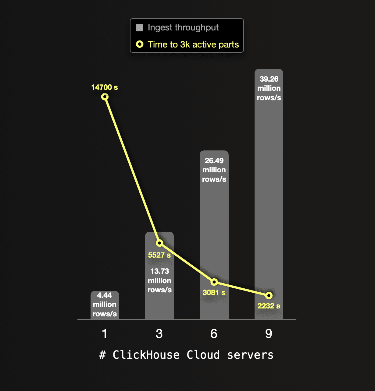 For each ingestion test run, we used the optimal tuning settings (32 parallel insert threads with an insert block size of 10 million rows) identified in the section above.
We can see that the ingest throughput scales perfectly linearly with the number of CPU cores and ClickHouse servers, respectively. This enables us to run your large data inserts as fast as you want.
It can be as fast as you want it to be
ClickHouse Cloud allows you to easily scale ingest duration linearly with additional CPU cores and servers, respectively. Therefore, you can run large ingests as fast as required. The following chart visualizes this:
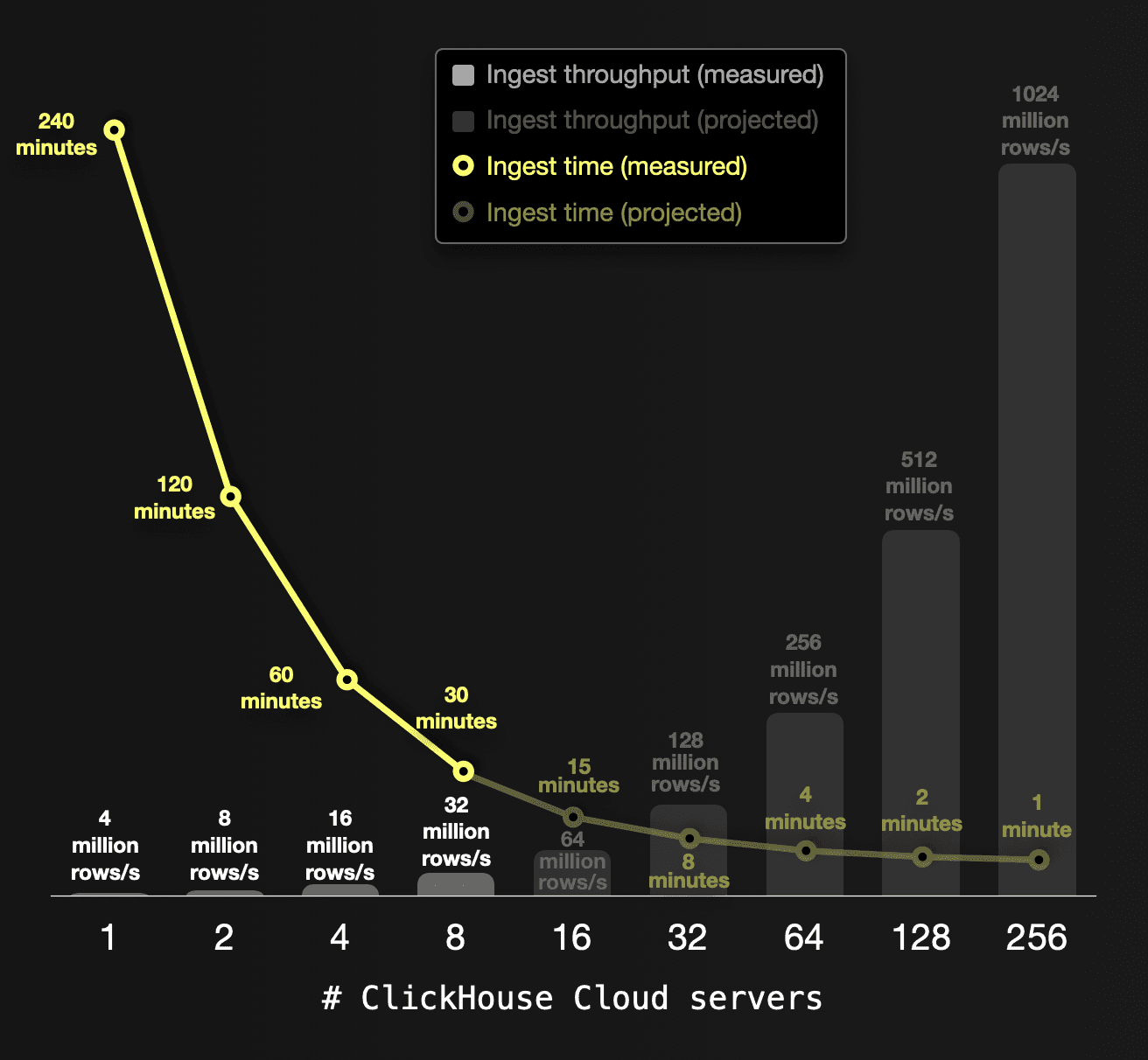 A single ClickHouse Cloud server (with 59 CPU cores and 236 GB RAM) ingests our 65 billion row dataset with a throughput of ~4 million rows per second in ~240 minutes. Based on our ingest test runs above proving linear scalability, we project how the throughput and ingest time can be improved with additional servers.
Summary
In this second part of our three-part blog series, we gave guidance and demonstrated how to tune the major insert performance factors for drastically speeding up a large multi-billion row insert. On the same hardware, the top ingestion speed is almost 3 times faster than with default settings. Additionally, we utilized ClickHouse Cloud’s seamless cluster scaling to make the ingest even faster and illustrated how you can run your large data inserts as fast as you want by scaling nodes.
We hope you learned some new ways to supercharge your large ClickHouse data loads.
In the next and last post of this series we will demonstrate how you can load a large dataset incrementally and reliably over a long period of time.
Stay tuned!


